Unleashing the Power of Machine Learning: A Step-by-Step Demo on QuantConnect
In this blog post, you will get a hands-on demonstration of machine learning techniques using the powerful QuantConnect platform. Whether you’re a seasoned developer, a data enthusiast, or just someone curious about the potential of machine learning, this demo will leave you inspired and eager to explore the limitless possibilities of this cutting-edge technology. Get ready to witness firsthand how machine learning can revolutionize trading strategies, optimize investment decisions, and unlock hidden patterns in financial data.
Table of contents
- A Primer on Machine Learning
- The Method
- Choosing a Machine Learning Library
- Creating Subscriptions
- Building Models
- Training Models
- Predicting Labels
- Managing Models
A Primer on Machine Learning
Machine Learning (ML) algorithms build a model based on sample data, known as training data, in order to make predictions or decisions without being explicitly programmed to do so. In this section, I will briefly cover some ML algorithms to help get a sense of how they work. If you want to follow along by coding your own examples, a popular library for testing different ML algorithms in python is sklearn.
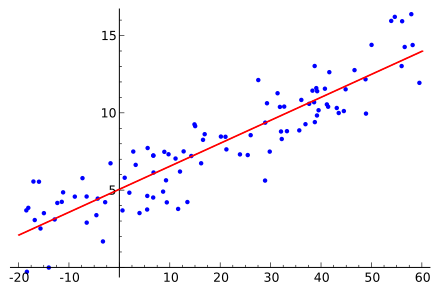
The simplest form of ML, in my opinion, is linear regression. A single line is drawn that minimizes the distance to all points in a dataset. You can find an implementation of this in sklearn as well as some examples. When applying linear regression to trading, the basic assumption is that the variance of the residual errors is constant. For instance, pricing data during a consistent bull market would meet this requirement, but would not if we added pricing data from a bear market as well. (there are a lot of caveats here as I’m trying to keep it simple)
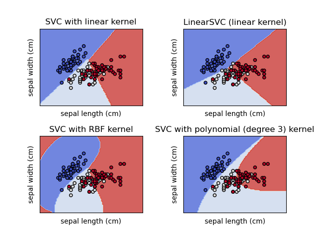
Support vector machines (SVM) are supervised learning models that analyze data for classification and regression analysis. SVM builds a model that assigns data points to a category. You can find an implementation and examples in the sklearn library. In the diagram, you can see how different kernels allow data points to be classified with increasing degrees of precision. I’ve used SVM to determine securities that would increase in a given quarter based on prior quarters’ fundamental data.
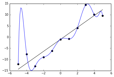
Although there are many more algorithms, I’ll finish this short primer by touching on the topic of overfitting. Generally speaking, when too much training is applied to a model or a model is too complex for a data set, it will approximate the training data too closely. This will decrease its performance when predicting out of sample data. For instance, if I apply a polynomial algorithm to data that only has a simple linear relationship, there is a higher chance of overfitting as you can see in the image.
The Method
Most ML trading implementations will follow the steps outlined in this hands-on demo. This blog post will start with the Hmmlearn example provided by Quantconnect. Further posts will develop on this one to go deeper into ML algo trading. Hmmlearn is a set of algorithms for unsupervised learning and inference of Hidden Markov Models.
Choosing a Machine Learning Library
The first step is choosing a ML library. Typically, I will do my data exploration within the Research environment provided with Quantconnect primarily because of the data available to me on the platform. If you do research in a different environment, make sure that the library you use is supported by Quantconnect.
Inserting the library is straightforward. We will also add the ‘joblib’ library to have a lightweight pipeline.
from AlgorithmImports import *
from hmmlearn import hmm
import joblib
Creating Subscriptions
The next step is subscribing to some data to train the hmmlearn model and make predictions. In the Quantconnect environment, basic data is included free of charge. Subscription means to selectively include the data in the running of the algorithm. Here, we will work with the SPY security, an ETF tracking the S&P500.
self.symbol = self.AddEquity("SPY", Resolution.Daily).Symbol
Building Models
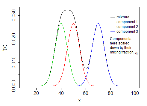
In this example, let’s assume the market has 2 regimes and the market returns follow a normal distribution. Without going into too much detail (because I don’t understand the depth of it), the components of the HMM will create a mixture that approximates our data.
self.model = hmm.GaussianHMM(n_components=2, covariance_type="full", n_iter=100)
Training Models
The initial training requires a history of data in order to complete successfully. The training length is expressed in days and I use a RollingWindow to maintain the history of data.
training_length = 252*2
self.training_data = RollingWindow[float](training_length)
history = self.History[TradeBar](self.symbol, training_length, Resolution.Daily)
for trade_bar in history:
    self.training_data.Add(trade_bar.Close)
With the price data ready, it’s time to train the model. Before ‘fitting’ (training) the model, I will create the feature of daily percent change.
def get_features(self):
    training_df = np.array(list(self.training_data)[::-1])
    daily_pct_change = (np.roll(training_df, 1) - training_df) / training_df

    return daily_pct_change[1:].reshape(-1, 1)

def my_training_method(self):
    features = self.get_features()
    self.model.fit(features)
Typically, I will retrain a model periodically to capture any changes in market conditions. Best practice is to retrain models outside business hours. Keep in mind that training time is limited in live algorithms (30 minutes at the time of writing), after which time the algorithm will timeout. If your training is longer than this, I would suggest you train the model in the Research environment, save it, and then restore it in the live environment.
self.Train(self.my_training_method)
self.Train(self.DateRules.Every(DayOfWeek.Sunday), self.TimeRules.At(8, 0), self.my_training_method)
As the live algorithm progresses in time, we need to update the RollingWindow.
def OnData(self, slice: Slice) -> None:
    if self.symbol in slice.Bars:
        self.training_data.Add(slice.Bars[self.symbol].Close)
Predicting Labels
Most of the work is done in the model training step. At this point, we can simply predict our feature using the trained model.
new_feature = self.get_features()
prediction = self.model.predict(new_feature)
prediction = float(prediction[-1])
The prediction is then used as a signal to place orders.
if prediction == 1:
    self.SetHoldings(self.symbol, 1)
else:
    self.Liquidate(self.symbol)
Managing Models
Models can be saved and restored between algorithm runs. For instance, this can be useful when training the model separately in the Research environment due to the length of fitting. Or, this can act as a means to accelerate the startup of an algorithm by avoiding to initialize the history of data.
Conclusion
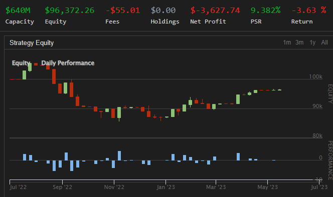
The backtesting results at -3% are rather poor in my opinion. I would look at changing certain parameters such as the history length, the model configuration, and perhaps changing ML algorithm. This was meant as a demonstration, not investing advice.
In this post, I presented a short primer to ML algorithms, followed by a series of steps as a basic method to use most ML algorithms in trading. Take your time building on these steps as you will develop your own specific method. Accessing the power of ML in your trading will unlock an incredible number of possibilities for your strategies.
